Results
Contents
Results
Progress overview
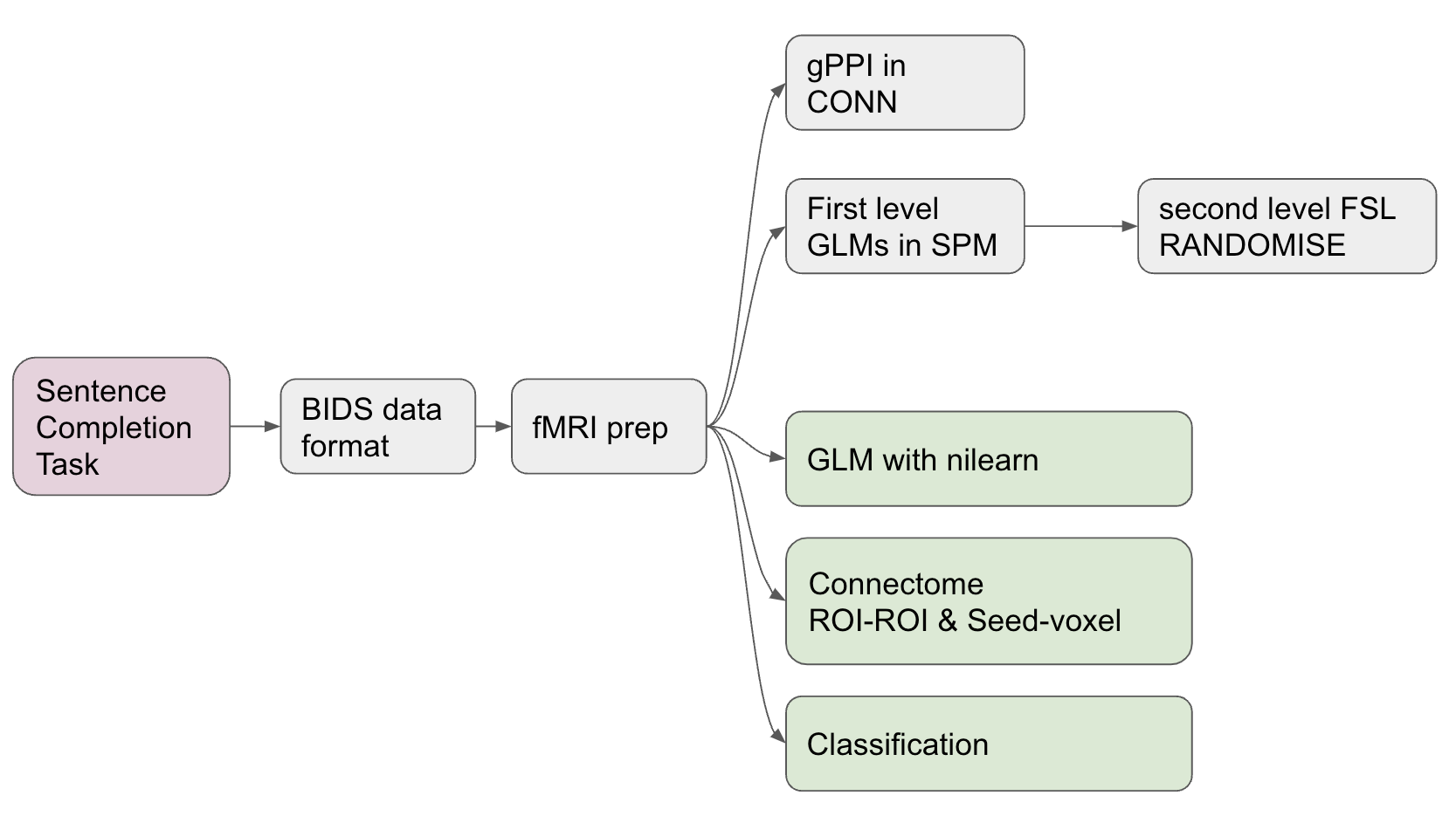
The brainhack school provided four weeks of space during which I could work full time on the analysis of this Tulpa dataset. At the end of these four weeks I was able to complete a first draft of all major analyses intended. These analyses include:
GLM (first and second level).
Task related connectivity.
ML classifier to differentiate conditions using the connectome;
A deep learning decoding appraoch using PyTorch to distinguish the task conditions.
Tools I learned during this project
This project was intended to upskill in the use of the following
Nilearnto analyse fMRI data in python.Scikit-learnto realise ML classification tasks on fMRI related measures.Py Torchto implement a brain decoder.Jupyter {book}andGithub pagesto present academic work online.Markdown,testing,continuous integrationandGithubas good open science coding practices.
Results
Deliverable 1: project report
You are currently reading the project report.
Deliverable 2: project website
In addition to this report, I made a github website. However, please note that the website does not currently show the full report of this project as the publication is waiting for final approval from the Principal Investigator of this project.
This project website was created using Jupyter {books}. This format allows for a potential submission to neurolibre. Neurolibre is a preprint server for interactive data analyses.
Deliverable 3: project github repository
The repository of this project can be found here. The objective was to create a processing pipeline for ECG and pupillometry data. The motivation behind this task is that Marcel’s lab (MIST Lab @ Polytechnique Montreal) was conducting a Human-Robot-Interaction user study. The repo features:
a video introduction to the project.
a presentation made in a jupyter notebook on the results of the project.
Notebooks for all analyses.
Detailed requirements files, making it easy for others to replicate the environment of the notebook.
An overview of the results in the markdown document.
Deliverable 4: GLM results
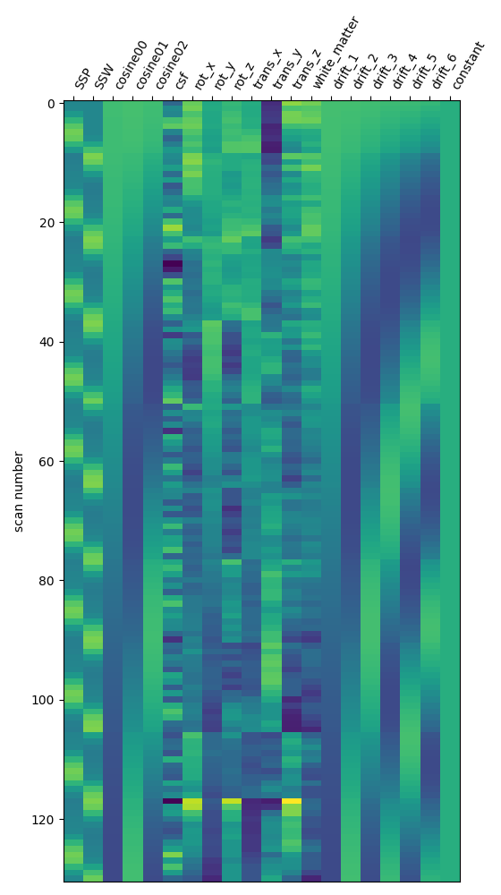
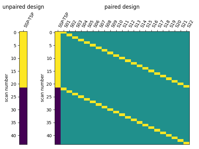
I have used Nilearn to compute a GLM that compares different conditions of the task. Specifically, I am interested in teh respective contrasts between self, tulpa, and friend. I am interested in these contrasts for the preparation and writing phase respectively. I have computed the GLM on fmriprep prepreocessed data. I have then created a design matrix that integrates the timing files (first two columes) as well as well as some movement regressors (see figure below). To incorporate the movement regressors I have used the load_confounds_strategy from nilearn with the following parameters: denoise_strategy="scrubbing", motion="basic", wm_csf="basic".
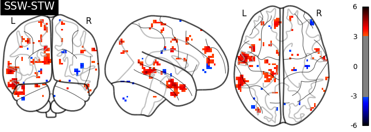
I have then computed a second level analysis that combines the individual beta maps into a group level contrast between the different conditions (see design matrix below). As a result I receive z-scores of each voxel, indicating how much that voxel differs across the two compared condition. The plot below displays these z-scores for comparing the self-write with the tulpa-write condition. A z-score of 3.0 is equivalent to a 99% confidence interval, a z-score of 2.3 is equivalent to a 95% confidence interval.
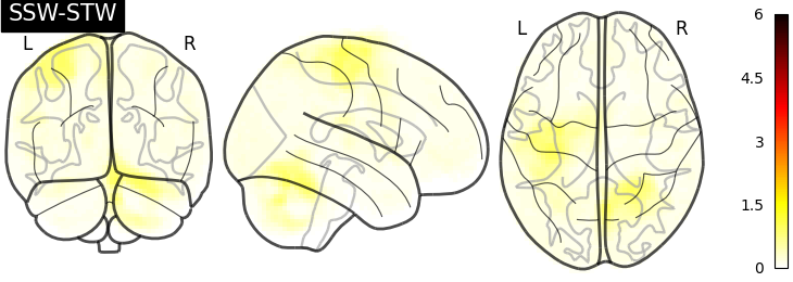
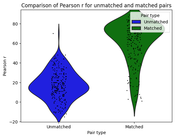
I then used Neuro Maps to compute the pearson-r correlation between the first level outputs computed with Nilearn to those I previously computed with SPM. To test for the significance of these comparisons, I re-computed the pearson-r for random pairs. The r values of the true (matched) pairs have a mean of 61.32 while the mean of the random (unmatched) pairs is 17.09. A two-sample t-test revleaed that this difference is significant: T-stat: -26.24 and a p-value=0.000.
:information_source: matched pairs are between software, within subject, within contrast, within run.
:information_source: unmatched pairs are between software, between subject, between contrast, between run
Deliverable 5: Connectome results
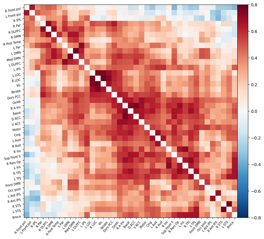
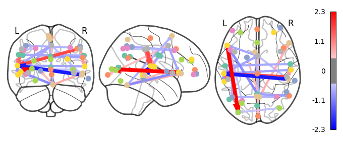
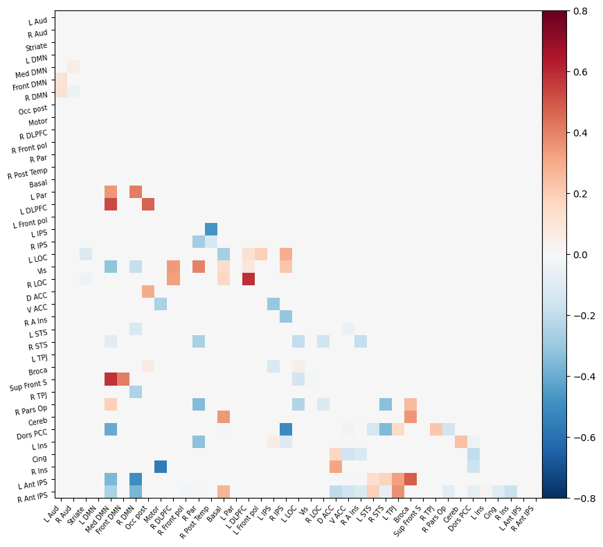
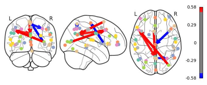
I have parcellated the brain into 39 regions based on the probabilistic msdl atlas. A probabilistic atlas assigns a probability to each voxel, indicating how likely it is that that voxel belongs to a specific region. I have then computed the correlation between all of these 39 regions, resulting into a connectome of shape 39*39. Given that that the correlation measure is none directive, the upper and lower triangle of the connectome mirror each other. Below is an example of a connectome for one subject and one condition.
Deliverable 6: Seed-to-Voxel connectivity results
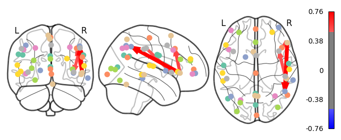
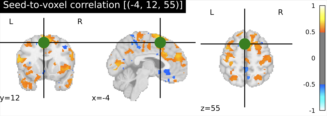
I have previously computed a gPPI for this dataset using CONN. I wanted to replicate this task dependent seed to voxel correlation using Nilearn. I have specified the seed based on the group peak activation in the SMA, using the results from the SPM and Randomise analysis. Seed coordination in MNI space are (-4, 12, 55). I have then constructed a sphere around this voxel with a radius of 5 mm. Using this ROI, correlations to all voxels based by task condition were computed. Below is an illustrative example of the connectivity values for one subject and one condition.
Deliverable 7: ML-classifier results
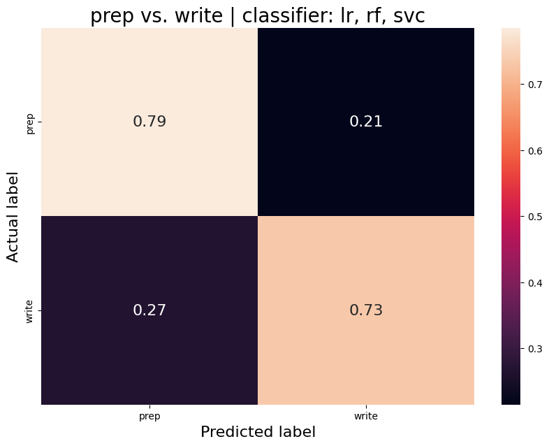
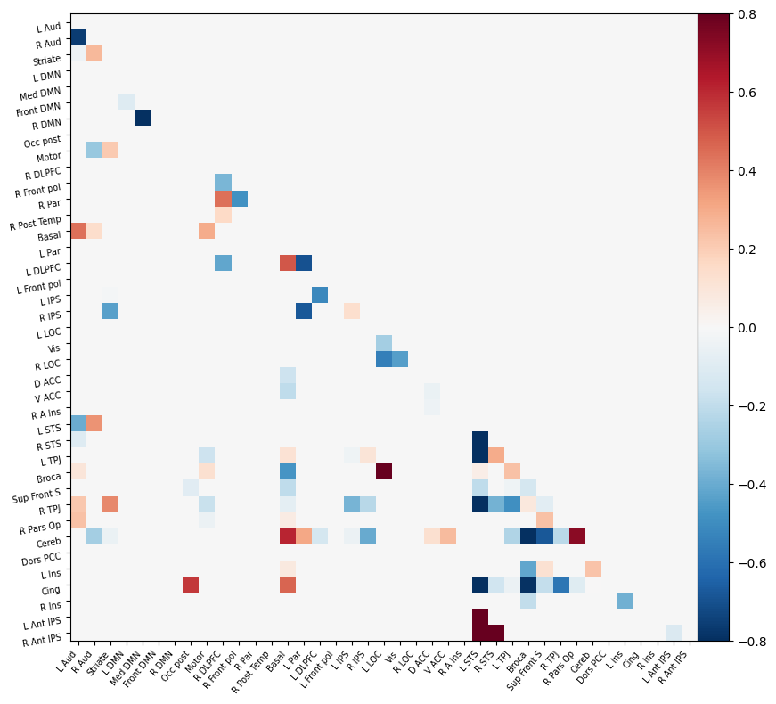
The aim was to train a classifier that can accurately distinguish between different task conditions. I used a majority vote ensemble classifier that combines LogisticRegression, RandomForestClassifier, and a SVC. When classifying the conditions prep vs. write, the classifier achievs an acciracy of ~80%, so well above chance. However, this is not surprising as the writing conditions will have muhc stronger motor cortex activation and the two conditions are quite different. I then classified the self, tulpa, and friend conditions for preparation and writing respectively. In both conditions, we have an accuracy of ~51% for this 3-group classification problem. Given the three groups, chance levels are at 33.3%, thus an accuracy of 51% is well above chance, YAY!
:information_source: all classifiers were trained and tested on the connectome. Next, the plan is to train classifiers on the beta maps of the GLM. See my to-do list for further details.
Prep-write condition
Average accuracy = 0.76
P-value (on 100 permutations): p=0.00
Write condition
Average accuracy = 0.52
P-value (on 100 permutations): p=0.32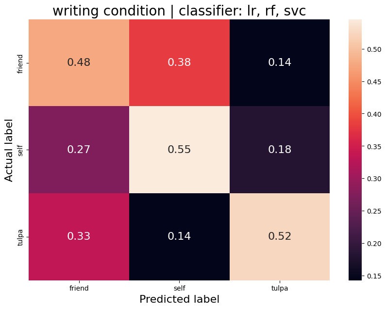
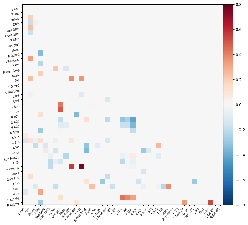
Prep condition
Average accuracy = 0.37
P-value (on 100 permutations): p=0.00
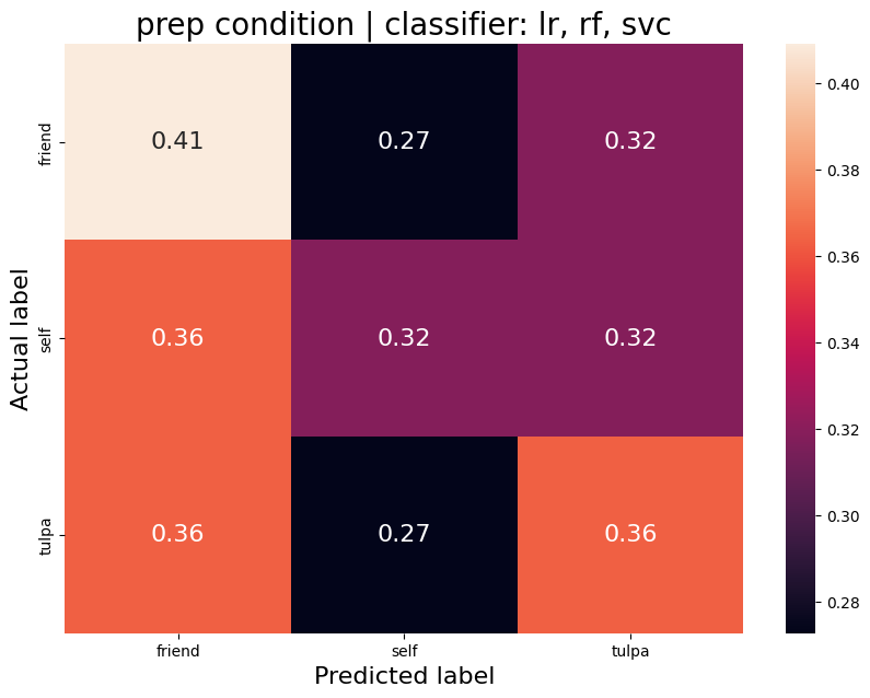
Deliverable 8: Deep neural network encoding results
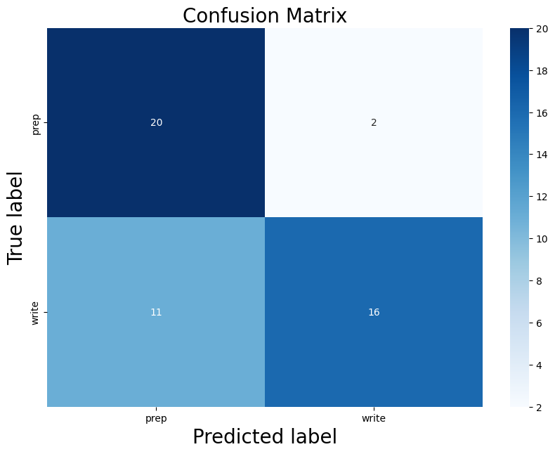
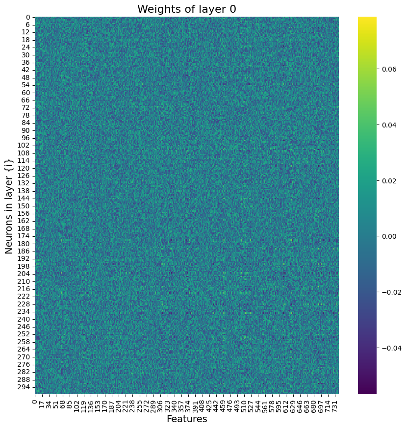
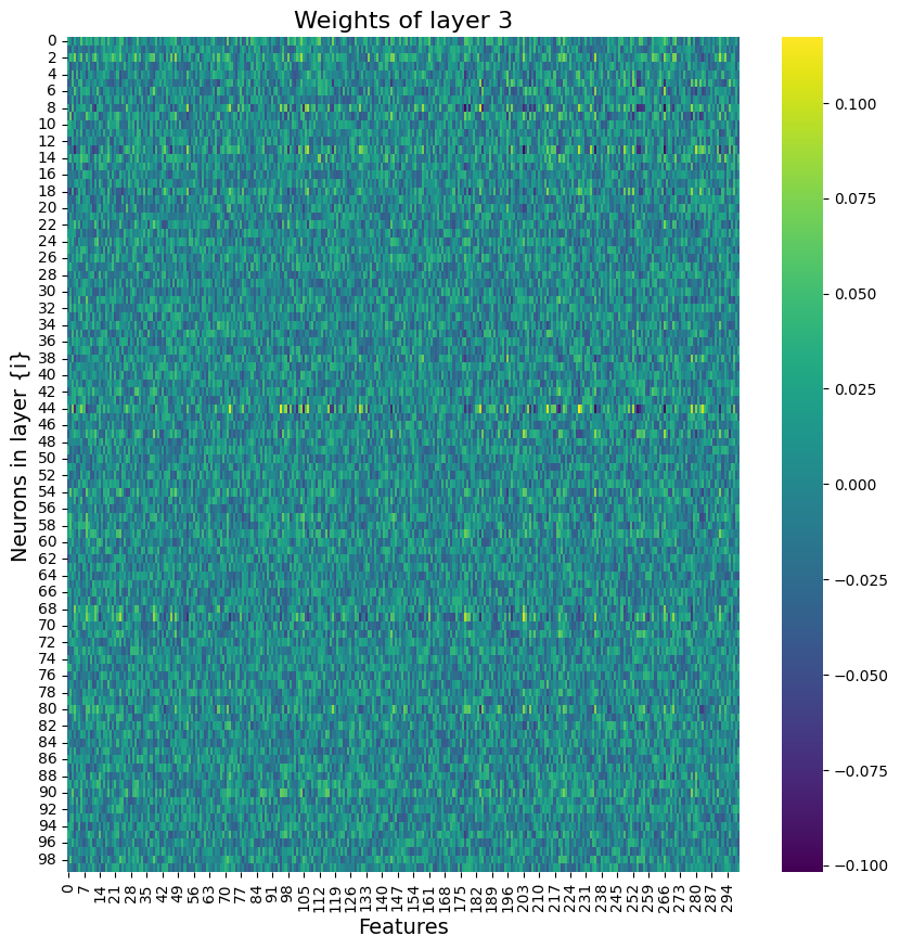
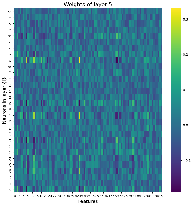
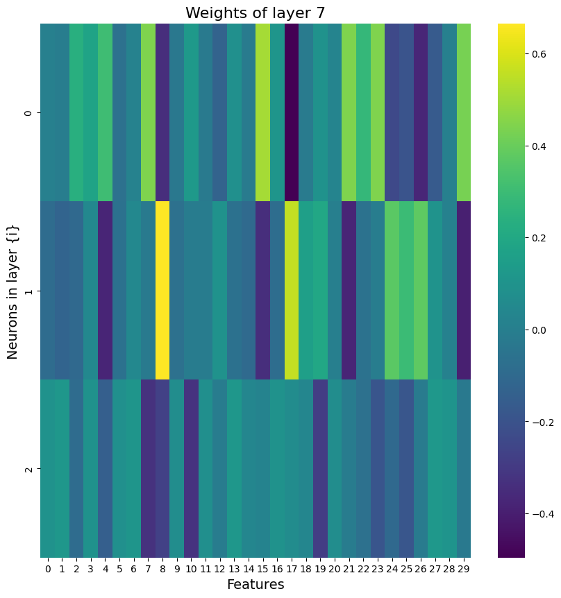
Building on what I have done with the ML classifiers, I wanted to explore if I could achieve the same resutls with a Neural Netowrk. I used PyTorch to build a Multilayer Perceptron with 4 linear layers, 3 rectified linear unit, and one dropout layer with a threshold of 0.3. I then trained this model with a learning rate of 0.01 and a weight decay of 0.01. The results show an accuracy of 0.73 which is simialr, though slightly lower, than the accuracy of the scikit learn ensemble classifier of 0.76.
Below you can see the definitino of the model, the confusion matrix, the learning rate of the model, as well as the weights of the trained model.


